The IDV has the ability to make quantities computed through the use of formulas available under the loaded data source rather than going through the steps to use a formula, as outlined in the previous section. For example, you could compute wind speed using the formula directly — simply load a Data Source, then from the Field Selector click Formulas→Workshop→Windspeed from u and v data, then click Create Display, then choose the fields for u and v and THEN you're done. Wouldn't it be nice if the IDV could recognize the u and v fields in your dataset and automatically present you with the choice to display Flow Vectors from u and v next to the available fields listed in your dataset? Well, this is exactly what Derived Quantities in the IDV accomplish.

Derived quantities can be created by doing the following:

1. Defining an IDV formula by name, description, and mathematical formula.
2. Using special operators (D1, D2, ... DN) for the variable names.
3. Specifying the binding between the special operators and the parameters names or system aliases.
4. Saving the formula and loading or reloading a data source.

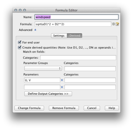
In the last section we discussed how to create a new Jython formula for wind speed, so the first step is complete. Now, let's examine how to turn our wind speed formula into a derived quantity. Let's open our wind speed function in the Forumla Editor by selecting the Edit→Formulas→Edit Formulas→Workshop→wind speed from u and v menu item. This brings up the Formula Editor dialog box we previously used to edit a formula. In this box, click the Derived tab to begin the process of enhancing the wind speed formula to produce derived quantities:

1. Click the Derived tab.
2. In the Formula, change u and v to D1 and D2, respectively. Note that the order of the parameters listed in the Parameters box is the same as the order used in the formula (i.e. D1 is U, D2 is V).
3. In the Parameters box, select the drop down list on right side and choose Aliases→Group #1→U component of wind (U) and Aliases→Group #2→V component of wind (V). Note that Group #1 and Group #2 do not correspond to the 1 and 2 in D1 and D2. The "1" and "2" in the D# variables are associated with the order of the parameters listed in the Parameter box; using groups in the alias list helps keep the list from becoming too long to display in the GUI.
4. click Change Formula

If we reload our data sources (right click on the data source in the Filed Selector and click reload), we will see a new category of data listed in the fields panel called Workshop, which when expanded contains our wind speed function.

There are other properties you can assign to your derived quantity, but this is the minimum effort needed to get things working (for more information, see Derived Products in the Users Guide).

Sometimes the IDV will not recognize the variables in your file, and thus will not be able to associate D1 with U because it does not know the name of the u component of velocity in your data set. In order to get the IDV to recognize the variables in your dataset, you may need to edit the Parameter Aliases. Click Tools→Parameter Alias Editor, then select System Aliases. Here you will find a list of Names (which are those used in the Parameters box in the Formula Editor), descriptions, and variable names associated with each Name.

For example, let's say you have a dataset in which the u component of velocity is called 'UCOMPWIND'. If we double click on the "U" name, the Alias Editor will automatically add a copy of the "U" alias to our User Aliases list and prompt us to add a new name to the alias list.

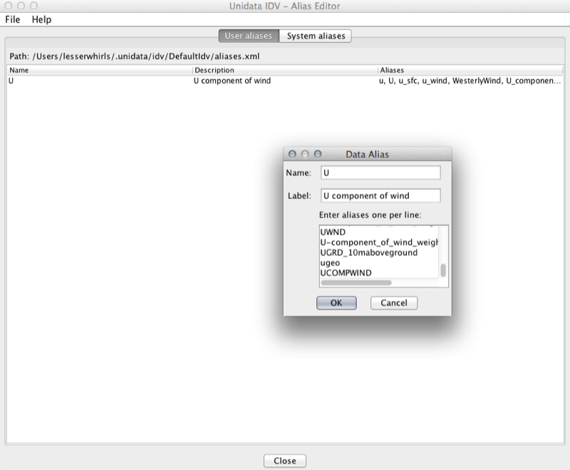
Once UCOMPWIND is added to the alias list, the IDV will know to associate UCOMPWIND with the U variable used in derived quantities. Changes to the alias list also apply to the system derived quantities, such as:

• Dewpoint
• Mixing ratio
• Relative Humidity
• Dewpoint Depression
• Equivilent Potential Temperature
• Potential Temperature
• Horizontal Divergence
• Relative Vorticity
• Height from Geopotential
• Isentropic Potential Vorticity
• Geostrophic Wind Vectors
• Ageostrophic Wind Vectors
• Wind Speed
• 3D Flow Vectors
• True Wind Vectors
• Ocean Flow Vectors
• Sounding Data (with and without winds)

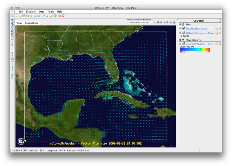
The IDV allows for one parameter to be colored by another parameter's value through the use of a formula. For example, let's view wind vectors colored by temperature:

1. Clear any existing displays by clicking the red and white eraser symbol found just below the Main Menu bar on either the Dashboard to Main View window.
2. Make sure your WRF ouput is loaded.
3. In the Field Selector panel, select Formulas as the Data source and expand the Grids tab. Then, select the One value colored by another formula, choose the Flow Displays→Vector Plan View display, and click Create Display
4. For the data field choice, click on your WRF output and select 3D→Derived→True Wind Vectors (from u_wind & v_wind)
5. For the Color field, select 3D→Temperature @ isobaric and click OK
6. From the Displays tab, select coloredByAnother - Vector Plan View and set the Skip: XY: factor to 5
7. Click the button next to Color Table and select Change Range. Click the Use Predefined button and select From Displayed Data and click OK.

You can change the level at which the colored vectors are displayed directly from the Displays tab using the Levels drop-down box.

The IDV can generate 2D and 3D trajectories. To access the trajectory features:

1. Load your WRF data
2. In the Field Selector, select the Formulas data source and click Grids→Create 3D Flow Trajectory
3. Next, you will be prompted to select grids for u, v, w, s, and s0)

The fields of u, v, and w are the individual components of the wind. The field s is the field you would like to use to color the trajectory. The field s0 is special — the field itself isn't actually used, but the spatial subset defined in its Region tab is used. As the resources used to hold the data for trajectory computation are quite large, it's useful to spatially subset where you would like the trajectories to initiate. A good way to go about this is to use the same field for S and S0, but use the Region tab to subset S0 over the area of interest. Note that this is a new feature in the IDV and the user interface is likely to change!

That said, loading the data and computing the trajectories can be quite time consuming, so we've created an IDV bundle that will allow you to explore the trajectory capabilities of the IDV. The bundle can be found on the memory stick given to you as part of this course. However, it can also be found on our RAMADDA server if you are working through this tutorial at home.

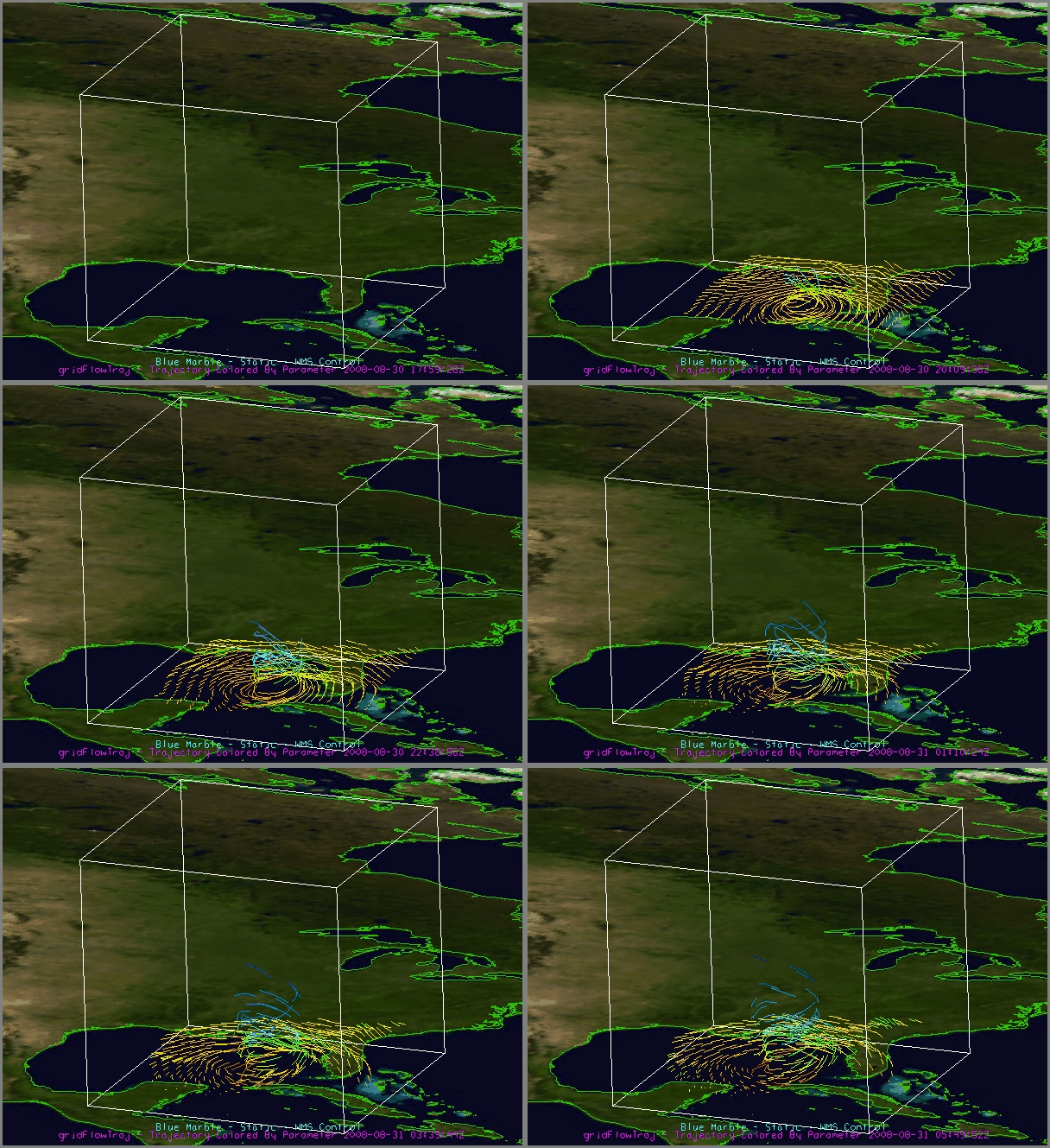
Use the IDV to load the GustavTrajectory.zidv bundle (located under the bundles folder on your memory stick) and explore the trajectory facility of the IDV. Note that it takes about 3 minutes on a high-end machine to create the display, so please be patient!

• From the main menu bar, click File→Open.
• Use the file dialog box to navigate to your bundle, and select your bundle.
• An Open bundle dialog box will appear — make sure Remove and displays & data and Try to add displays to current windows are checked and click OK.

The IDV contains many functions designed for analysis of ensemble model data. These functions can be utilized if the data you are using contains an ensemble dimension (alongside temporal and spatial dimensions). The ensemble functions can be accessed in the Field Selector panel by choosing "Formulas" as the Data source and expanding the Grids tab; The ensemble functions will be listed under the Ensemble tab.

Current ensemble functions include:

• Average over members
• Maximum over members
• Minimum over members
• Mode of the members
• Standard deviation of members
• Percentile calculation
• Range of values
• Univariate probability

The subsetting feature of the IDV can also be used to include/exclude specific members from these calculations.

Unidata IDV Workshop for version 6.3 > Accessing and Displaying Data > Working with WRF Output > Interactive