| 2.4.0 | Connecting to a Remote Server for a grid coverage type data |
| 2.4.1 | Cross Boundary Spatial Subsetting |
| 2.4.2 | To make a cross boundary 3D plot of GFS one degree data |
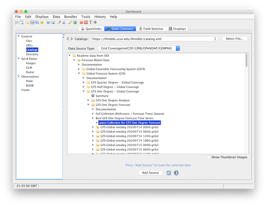
Choose one of the remote Catalogs:
such as https://thredds.ucar.edu/thredds/catalog.xml
of Unidata's Thredds Data Server for the near real-time model output.
A tree view of the catalog will be displayed. Open one, such
as the "GFS One Degree - Global Coverage model data (real and near time)",
by clicking on one of the tab icons
( ).
).
Specify the data source type to be Grid Coverage(netCDF/GRIB/OPENDAP/GEMPAK)
using the Data Source Type drop down menu. The IDV defualts the type
of model data as Grid files(netCDF/GRIB/OPENDAP/GEMPAK).
Only the "Grid Coverage" type has the feature of cross boundary spatial subset.
The list of this model's run times appears. Click on "Best Time Series" or "Latest Collection" to select it, and then click on the Add Source button. You have selected the model output to be accessible by the IDV.
Spatial Subset tab of
the Data Source Properties or the Field Selector. This works similarly to
the grid file subset where you can set properties for all fields of the Data Source or
override the default property for a particular field on the field selector subset panel.
The difference in the Coverage data spatial subset is that the Flip map longitude button
at the bottom of the panel will allow user to flip longitudes in a cyclic rectilinear grid from
0/360 to -180/180 (or vice-versa) before performing the cross boundary spatial subset.
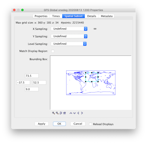
For more information on time and spatial subsetting, see the Data Source Properties page of this User's Guide.
)
to expand that category, further expand Momentum and
Derived tab, click on "Speed (from u-component_of_wind_isobaric &
u-component_of_wind_isobaric)" and select "Isosurface" display type,
click on the Create Display button to create a wind speed isosurface display. Create another
Contour Plan View in the Plan Views Displays list. Both displays will be created and shown in the main window.